This seminar note explores the geometric foundations of OLS, GLS, and GMM estimators through the lens of inner product spaces. We compare their respective objective functions as quadratic forms, analyze their level sets, and demonstrate how positive definite kernels reshape the geometry of estimation. By drawing parallels to Einstein’s field equations, we highlight how the structure of estimation reflects deeper principles of information weighting and spatial deformation.
Keywords
OLS, GLS, GMM, inner product space, positive definite kernel, Mahalanobis norm, projection geometry, quadratic form, estimation theory, level set visualization, Einstein field equations, metric tensor, heteroskedasticity, moment conditions
Inner Product, Projection, and the Role of Positive Definite Kernels
1 OLS as Orthogonal Projection in Euclidean Space
OLS solves the following problem:
\[
\hat{\beta}_{OLS} = \arg\min_\beta \| y - X\beta \|_2^2 = (X^\top X)^{-1} X^\top y
\]
This corresponds to projecting \(y\) orthogonally onto the column space of \(X\).
The residual \(\varepsilon = y - X\hat{\beta}\) satisfies:
\[
X^\top \varepsilon = 0
\]
1.1 Inner Product and Geometry
The \(L^2\) norm used in OLS is induced by the standard Euclidean inner product:
\[
\langle u, v \rangle = u^\top v
\]
The distance function becomes:
\[
\| u \|_2 = \sqrt{u^\top u}
\]
The set of parameter values yielding equal error defines a level set (isocurve):
\[
\{ \beta \mid \| y - X\beta \|_2^2 = c \} \Rightarrow \text{spheres in parameter space}
\]
This reflects Pythagorean geometry — the isocurves are circles (in 2D), spheres (in 3D), or hyperspheres in higher dimensions when \(X^\top X = I\); otherwise, elliptical.
In this sense, OLS performs Euclidean projection onto a linear subspace using the standard inner product.
2 Generalized Least Squares (GLS)
GLS extends OLS by accounting for non-spherical error covariance structure:
Here, \(\Sigma\) is the covariance matrix of the errors.
This defines a new inner product over the residual space:
\[
\langle u, v \rangle_\Sigma = u^\top \Sigma^{-1} v
\]
The level sets:
\[
\{ \beta \mid (y - X\beta)^\top \Sigma^{-1} (y - X\beta) = c \} \Rightarrow \text{ellipsoids in parameter space}
\]
This reflects how different directions in parameter space are penalized differently depending on the variance and correlation structure of the errors.
The ellipsoidal level sets visualized earlier correspond precisely to this GLS structure.
3 GMM as Orthogonality of Moment Conditions (Not Projection)
GMM generalizes the estimation framework by relying on moment conditions, not residuals:
\[
\hat{\theta}_{GMM} = \arg\min_\theta \left[ \bar{g}_n(\theta)^\top W \bar{g}_n(\theta) \right]
\]
where:
\(\bar{g}_n(\theta) = \frac{1}{n} \sum_{i=1}^n g(Z_i, \theta)\) is the sample mean of moment functions
\(W\) is a positive definite weighting matrix, usually the inverse of the estimated variance of \(\bar{g}_n(\theta)\)
3.1 Clarifying the Inner Product
Although GMM also defines a quadratic form like GLS, it operates in a fundamentally different space:
In GLS: \(u, v\) are residual vectors
In GMM: \(u, v\) are moment function evaluations
Thus, while one can write:
\[
\langle g_i(\theta), g_j(\theta) \rangle_W = g_i(\theta)^\top W g_j(\theta)
\]
it is important to emphasize:
GMM is not a projection-based method. It minimizes the violation of moment orthogonality conditions in expectation.
The isocurves:
\[
\{ \theta \mid \bar{g}_n(\theta)^\top W \bar{g}_n(\theta) = c \}
\]
may also appear elliptical — but they are not projections, and should not be conflated with GLS geometrically.
3.2 Local Approximation and Connection to GLS
In some cases, GMM can be viewed as a local GLS approximation. If moment conditions are close to linear in \(\theta\), and \(g(Z_i, \theta) \approx A(Z_i)(\theta - \theta_0)\), then the GMM objective becomes:
\[
(\theta - \theta_0)^\top A^\top W A (\theta - \theta_0)
\]
which resembles GLS — but only locally and approximately.
Therefore, the geometric intuition of ellipsoids applies more precisely to GLS. For GMM, it’s a useful visual aid — but structurally distinct.
4 Einstein Field Equations and GMM: Structural Analogy
Einstein’s Field Equations (EFE) in general relativity:
\(T_{\mu\nu}\): Stress-energy tensor, representing energy and matter (matter-energy distribution)
\(G_{\mu\nu}\): Einstein tensor, encoding the curvature of spacetime (curvature)
\(R_{\mu\nu}\): Ricci curvature tensor
\(R\): Scalar curvature
\(g_{\mu\nu}\): Metric tensor, defining the inner product in spacetime and governing geodesics
4.1 Analogy to Estimation Frameworks
Feature
OLS
GLS
GMM
EFE (Physics)
Space
Euclidean
Covariance-weighted
Moment function space
Curved spacetime
Inner product
\(I\)
\(\Sigma^{-1}\)
\(W\) (moment-weighted)
\(g_{\mu\nu}\) (metric)
Optimization
Projection
Weighted projection
Moment orthogonality
Energy-curvature balance
Level sets
Circles
Ellipses
Ellipsoid-like
Lightcones / geodesics
4.2 Lightcones and Degenerate Conics
In EFE, the metric tensor \(g_{\mu\nu}\) defines how distances and angles are measured — it is the analogue of a positive definite kernel in GMM. The field equations determine how the geometry (curvature) of spacetime reacts to matter and energy. In this sense, spacetime is optimized or shaped in response to external inputs, just as GMM shapes its estimation space based on the kernel \(W\) and moment functions.
The level sets in general relativity are often visualized as lightcones — the surface separating causal influence from spacelike separation. Geometrically, a lightcone can be interpreted as the degenerate case of a conic section, where the quadric form:
\[
Q(x) = x^\top g_{\mu\nu} x = 0
\]
results in a pair of intersecting lines: this represents all null (light-like) directions emanating from a point. These are the boundary cases between time-like and space-like intervals, analogous to the way ellipsoids in GMM collapse into degenerate forms under singular kernel matrices.
Thus, in both GMM and EFE, the shape and degeneracy of level sets encode deep information about the underlying structure — whether it is a statistical model or the geometry of spacetime.
5 Summary
OLS performs Euclidean projection in a space endowed with the standard inner product.
GLS generalizes this using a positive definite kernel over the residual space, yielding ellipsoidal level sets.
GMM further generalizes the concept by applying positive definite weighting over moment function space, not residuals.
Geometric analogies (spheres and ellipsoids) are structurally valid for OLS and GLS, and visually helpful — but must be used with care in GMM.
All three frameworks share a unifying theme: geometry induced by positive definite structure.
“OLS and GLS estimate by projection. GMM estimates by aligning empirical moments. Einstein’s theory bends space to match mass — estimation theory bends geometry to match data.”
6 Visuals
6.1 OLS vs. GLS: Different Projections Under the Same Linear Model
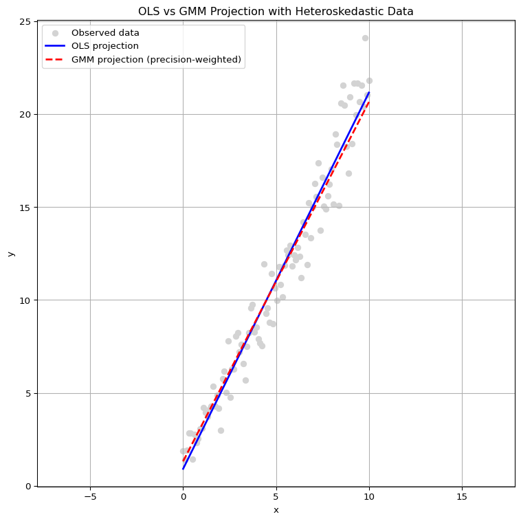
This section visualizes how OLS and GLS (with heteroskedastic weighting) yield different estimators even under the same linear model structure. The key distinction lies in how each method defines distance and importance via its respective inner product.
6.1.1 Simulation Setup
Data-generating process: \[
y = \beta_0 + \beta_1 x + \varepsilon
\] where the noise term \(\varepsilon\) is heteroskedastic — its variance increases with \(x\).
That is, the reliability of observations decreases toward the right end of the domain.
OLS estimation:
Minimizes the unweighted squared residuals: \[
\min_\beta \| y - X\beta \|_2^2
\]
Assumes all observations are equally informative.
The projection balances the residuals across the entire domain, including high-noise regions.
GLS estimation:
Minimizes a precision-weighted residual norm: \[
\min_\beta (y - X\beta)^\top W (y - X\beta)
\] where \(W\) is a positive definite diagonal matrix with weights inversely proportional to the noise variance.
Observations with lower noise (on the left) are more heavily weighted.
The resulting projection is skewed toward the low-variance region, yielding a steeper estimated slope.
6.1.2 Interpretation
Even though both methods fit a linear model, they differ fundamentally in the geometry of projection: - OLS projects onto the column space of \(X\) using the standard Euclidean inner product. - GLS projects in a space where the residuals are measured using a Mahalanobis-type norm, effectively reshaping the loss geometry.
This difference becomes visually striking when we compare their fitted lines on heteroskedastic data — OLS follows the average trend, while GLS emphasizes the cleaner data and suppresses the noisy part.
Code
import numpy as npimport matplotlib.pyplot as plt# Simulate data with heteroskedastic noise (to favor GMM adjustment)np.random.seed(0)n =100x = np.linspace(0, 10, n)X = np.vstack([np.ones(n), x]).T# True modelbeta_true = np.array([1, 2])# Heteroskedastic noise: variance increases with xnoise_std =0.5+1.5* (x / x.max()) # ranges from 0.5 to 2.0y = X @ beta_true + np.random.normal(0, noise_std)# OLS estimationbeta_ols = np.linalg.inv(X.T @ X) @ X.T @ yy_hat_ols = X @ beta_ols# GMM weighting: inverse of variance (precision weighting)W = np.diag(1/ noise_std**2)# GMM estimation (optimal weighting under heteroskedasticity)XTWX = X.T @ W @ XXTWy = X.T @ W @ ybeta_gmm = np.linalg.inv(XTWX) @ XTWyy_hat_gmm = X @ beta_gmm# Plot with aspect ratio 1:1plt.figure(figsize=(8, 8))plt.scatter(x, y, color='lightgray', label='Observed data')plt.plot(x, y_hat_ols, label='OLS projection', color='blue', linewidth=2)plt.plot(x, y_hat_gmm, label='GMM projection (precision-weighted)', color='red', linestyle='--', linewidth=2)plt.title("OLS vs GMM Projection with Heteroskedastic Data")plt.xlabel("x")plt.ylabel("y")plt.axis('equal') # Set equal aspect ratioplt.legend()plt.grid(True)plt.tight_layout()plt.show()
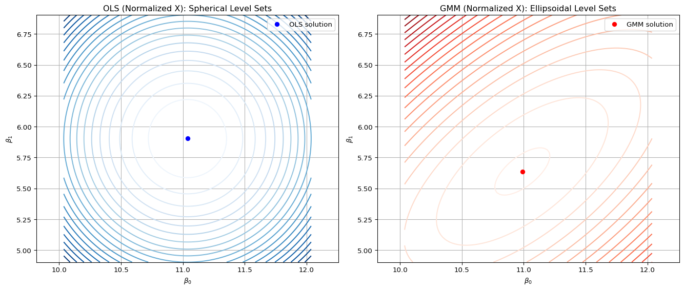
6.2 Different Level set of objective function (quadratic form)
Although the GLS objective has the same mathematical form as GMM, its geometry is defined over the residual space, not over the space of moment conditions.
The weighting matrix \(W\) in GLS is typically \(\Sigma^{-1}\), the inverse of the error covariance matrix.
Code
# ===============================================# GLS vs OLS: Visualization of Quadratic Forms## This code compares the level sets of:# (1) OLS objective (normalized via X'X)# (2) GLS objective with heteroskedastic weighting W## Although GLS and GMM share a similar quadratic structure,# this code reflects GLS estimation:# J(β) = (y - Xβ)' W (y - Xβ)# where W is a user-defined positive definite matrix (e.g., precision).## The level sets visualize how the estimation geometry is altered# under different inner products: Euclidean vs. Mahalanobis.# ===============================================# Z-score normalization of x to improve XtX conditionfrom sklearn.preprocessing import StandardScalerscaler = StandardScaler()x_normalized = scaler.fit_transform(x.reshape(-1, 1)).flatten()X_normalized = np.vstack([np.ones(n), x_normalized]).T# Recalculate OLS and GMM using normalized Xbeta_ols_norm = np.linalg.inv(X_normalized.T @ X_normalized) @ X_normalized.T @ yy_hat_ols_norm = X_normalized @ beta_ols_norm# GMM estimation with same WXTWX_norm = X_normalized.T @ W @ X_normalizedXTWy_norm = X_normalized.T @ W @ ybeta_gmm_norm = np.linalg.inv(XTWX_norm) @ XTWy_normy_hat_gmm_norm = X_normalized @ beta_gmm_norm# New grid around beta_ols_normb0_vals = np.linspace(beta_ols_norm[0] -1, beta_ols_norm[0] +1, 100)b1_vals = np.linspace(beta_ols_norm[1] -1, beta_ols_norm[1] +1, 100)B0, B1 = np.meshgrid(b0_vals, b1_vals)B_flat = np.vstack([B0.ravel(), B1.ravel()])# Normalized OLS objective (Mahalanobis)XtX_inv_norm = np.linalg.inv(X_normalized.T @ X_normalized)delta_norm = B_flat - beta_ols_norm[:, None]J_ols_normalized = np.einsum('ji,jk,ki->i', delta_norm, XtX_inv_norm, delta_norm).reshape(B0.shape)# GLS objective with normalized XJ_gmm_norm = []for i inrange(B_flat.shape[1]): r = y - X_normalized @ B_flat[:, i] obj = r.T @ W @ r J_gmm_norm.append(obj)J_gmm_norm = np.array(J_gmm_norm).reshape(B0.shape)# Plottingfig, axs = plt.subplots(1, 2, figsize=(14, 6))# Normalized OLS (should be spherical)cs1 = axs[0].contour(B0, B1, J_ols_normalized, levels=20, cmap='Blues')axs[0].plot(beta_ols_norm[0], beta_ols_norm[1], 'bo', label='OLS solution')axs[0].set_title("OLS (Normalized X): Spherical Level Sets")axs[0].set_xlabel(r"$\beta_0$")axs[0].set_ylabel(r"$\beta_1$")axs[0].axis('equal')axs[0].legend()axs[0].grid(True)# GLS with normalized Xcs2 = axs[1].contour(B0, B1, J_gmm_norm, levels=20, cmap='Reds')axs[1].plot(beta_gmm_norm[0], beta_gmm_norm[1], 'ro', label='GMM solution')axs[1].set_title("GMM (Normalized X): Ellipsoidal Level Sets")axs[1].set_xlabel(r"$\beta_0$")axs[1].set_ylabel(r"$\beta_1$")axs[1].axis('equal')axs[1].legend()axs[1].grid(True)plt.tight_layout()plt.show()