07 Robustness

Is TBTF Sadly Optimal by Design?

While the previous section focused on the performance outcomes of the TBTF strategy, this section evaluates the stability of those outcomes under variation in core implementation parameters. We test whether the superior performance persists under changes in portfolio size, rebalancing frequency, weighting schemes, and look-back windows.

Rather than relying on a single optimized configuration, the TBTF strategy demonstrates structural robustness across plausible alternatives. This not only reinforces the credibility of the results, but also supports the practical adaptability of the approach for different institutional contexts.

All robustness tests are performed on the post-2010 period, with out-of-sample investment beginning on 2010-01-01. The portfolio is trained using a 48-month rolling window (in_sample=48M) and evaluated through 2023-12-31.

import pandas as pd
import sqlite3
cons = sqlite3.connect(database="../../tbtf.sqlite")

crsp = pd.read_sql_query(
  sql="SELECT * FROM crsp",
  con=cons,
  parse_dates={"date"}
)

# Out-of-sample Investment
import sys
import os
# 현재 경로 기준으로 상위 디렉토리로 경로 추가
sys.path.append(os.path.abspath('../..'))

import tbtf


# robust check 대상 파라미터 설정
top_ns = [5, 7, 10, 15, 20]
rebalance_freqs = ['3M', '6M', '12M']
weighting_methods = ['exponential', 'quadratic', 'value', 'equal']

# 기본 설정 정리
in_end = '2009-12-31'         # in-sample 끝
out_end = '2023-12-31'        # out-of-sample 끝
in_sample_months = 48         # in-sample 기간 (예: 4년)
eta = 3                       # CRRA 계수
p = 0.01                      # Omega Ratio threshold
state = 10


from joblib import Parallel, delayed

def run_single_backtest(method, n, freq):
    result = tbtf.backtest_pipeline(
        crsp=crsp,
        in_end=in_end,
        out_end=out_end,
        in_sample_months=in_sample_months,
        rebalance_freq=freq,
        weighting_method=method,
        top_n=n,
        state=state,
        eta=eta,
        p=p
    )
    perf = result['performance']
    perf.update({'n': n, 'rebalance_freq': freq, 'weighting_method': method})

    turnover_df = result['turnover']
    total_turnover = turnover_df.iloc[:-1]['turnover'].sum() if len(turnover_df) > 1 else np.nan

    return perf, {'n': n, 'rebalance_freq': freq, 'weighting_method': method, 'total_turnover': total_turnover}

from itertools import product

param_grid = list(product(weighting_methods, top_ns, rebalance_freqs))

# 병렬 실행
results = Parallel(n_jobs=-1)(delayed(run_single_backtest)(method, n, freq) for method, n, freq in param_grid)

# Robustness check 결과 DataFrame 생성
performance_df = pd.DataFrame([r[0] for r in results])
turnover_summary_df = pd.DataFrame([r[1] for r in results])

1 By Weighting Method

We begin by comparing the four weighting schemes: exponential, quadratic, value-weighted, and equal-weighted portfolios. The results show that TBTF’s convex weighting yields consistently superior risk-adjusted performance, particularly in terms of expected CRRA utility and downside-sensitive metrics like the Omega ratio. We set the CRRA parmater \(\eta = 3\) to reflect moderate risk aversion and \(p = 0.01\) to evaluate downside risk via the Omega Ratio at the minimum 1% monthly threshold.

metrics = ['Expected CRRA', 'Annualized Return', 'Sharpe Ratio', 'Sortino Ratio', 'Calmar Ratio', 'Omega Ratio', 'Max Drawdown']
performance_df.groupby('weighting_method')[metrics].median().round(3).sort_values(by='Expected CRRA', ascending=False)

Good Performance Metrics by Weighting Method

	Expected CRRA	Annualized Return	Sharpe Ratio	Sortino Ratio	Calmar Ratio	Omega Ratio	Max Drawdown
weighting_method
exponential	0.020	0.051	0.766	1.444	0.430	2.155	-0.134
quadratic	0.020	0.052	0.779	1.443	0.433	2.182	-0.132
value	0.020	0.050	0.770	1.454	0.435	2.147	-0.134
equal	0.018	0.045	0.727	1.326	0.382	1.967	-0.135

metrics = ['Annualized Volatility', 'Pearson Skewness', 'Excess Kurtosis']
performance_df.groupby('weighting_method')[metrics].median().round(3).sort_values(by='Annualized Volatility', ascending=True)

Bad Performance Metric by Weighting Method

	Annualized Volatility	Pearson Skewness	Excess Kurtosis
weighting_method
equal	0.064	-0.341	0.307
exponential	0.068	-0.240	0.752
value	0.068	-0.144	0.524
quadratic	0.069	-0.214	0.791

import seaborn as sns
import matplotlib.pyplot as plt

#sns.violinplot(data=performance_df, x='weighting_method', y='Annualized Volatility')
sns.boxplot(data=performance_df, x='weighting_method', y='Sharpe Ratio')
plt.title("Metric Distribution by Weighting Method")
plt.show()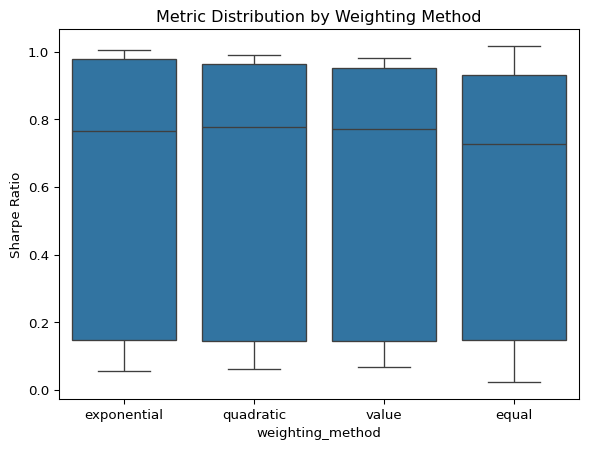

These results suggest that nonlinear weighting schemes are critical to capturing the TBTF premium. Among them, the quadratic method slightly outperforms exponential weighting across most performance metrics, including the highest median Omega ratio (2.182) and lowest median max drawdown (−13.2%). Given that both exponential and quadratic weighting schemes yield nearly identical results under the median of CRRA-based metrics, the exponential weighting—though rooted in CRRA-type concentration—offers no clear advantage over the quadratic scheme, which continues to strike a robust balance between concentration and diversification.

2 By Asset Selection Size (top_n)

Next, we vary the number of selected stocks, ranging from 5 to 20. The results clearly show that performance declines as top_n increases, confirming that capital concentration—not mere size exposure—is the key driver.

performance_df.pivot_table(
    values='Sharpe Ratio',
    index='weighting_method',
    columns='n',
    aggfunc='mean'
)

Sharpe Ratio by Weighting Method and Top-n

n	5	7	10	15	20
weighting_method
equal	0.608791	0.627588	0.605765	0.584674	0.585974
exponential	0.636665	0.648066	0.622787	0.604382	0.602568
quadratic	0.612236	0.642290	0.630014	0.610713	0.597321
value	0.616514	0.633672	0.615023	0.608970	0.605151

performance_df.pivot_table(
    values='Expected CRRA',
    index='weighting_method',
    columns='n'
).round(4)

Expected CRRA Utility across Weighting Methods and Top-n

n	5	7	10	15	20
weighting_method
equal	0.0168	0.0167	0.0141	0.0119	0.0110
exponential	0.0175	0.0174	0.0154	0.0135	0.0125
quadratic	0.0167	0.0172	0.0156	0.0138	0.0127
value	0.0166	0.0168	0.0151	0.0139	0.0130

Varying the number of selected stocks from 5 to 20 reveals a consistent trend: risk-adjusted performance tends to decline once the portfolio exceeds \(n=7\).

This pattern implies that the TBTF premium is not a gradual function of portfolio size, but instead concentrated at the extreme upper tail of the capital distribution. The declining marginal benefit of including additional assets reflects the structural nature of capital lock-in—only the very largest firms systematically attract persistent investor flows, benefit from narrative insulation, and receive reinforcement through index inclusion.

Notably, traditional weighting schemes (Value or Equal) consistently underperform compared to TBTF-based weightings (Exponential or Quadratic) when \(n < 15\), highlighting the importance of embedding size asymmetry in portfolio construction.

3 Rebalancing Frequency and Turnover Tradeoff

import seaborn as sns
import matplotlib.pyplot as plt

# 원하는 순서로 정렬
rebalance_order = ['3M', '6M', '12M']
n_order = sorted(performance_df['n'].unique(), reverse=True)  # n=5,7,10,15,20 등 오름차순

# Pivot and reorder
pivot_sharpe = (
    performance_df.pivot_table(
        values='Sharpe Ratio',
        index='n',
        columns='rebalance_freq'
    )
    .loc[n_order, rebalance_order]  # y축 (n), x축 (rebalance_freq) 순서 정렬
    .round(2)
)

# Pivot을 위한 사용자 정의 함수
def best_weighting_by_sharpe(df):
    idx = df.groupby(['n', 'rebalance_freq'])['Sharpe Ratio'].idxmax()
    best_df = df.loc[idx, ['n', 'rebalance_freq', 'weighting_method']]
    pivot = best_df.pivot(index='n', columns='rebalance_freq', values='weighting_method')

    # 시각화-friendly 정렬
    pivot = pivot.loc[sorted(pivot.index, reverse=True), ['3M', '6M', '12M']]
    return pivot

best_weighting_pivot = best_weighting_by_sharpe(performance_df)

# 결과 출력
# display(best_weighting_pivot)

plt.figure(figsize=(8, 5))
# sns.heatmap(pivot_sharpe, annot=True, cmap="YlGnBu", cbar_kws={'label': 'Sharpe Ratio'})
sns.heatmap(
    pivot_sharpe,  # 기존 numeric table
    annot=best_weighting_pivot.values,  # 텍스트는 scheme 이름으로
    fmt='',  # 숫자 포맷 아님
    cmap="YlGnBu",
    cbar_kws={'label': 'Sharpe Ratio'}
)
plt.title("Best Weighting Method by Sharpe Ratio")
plt.xlabel("Rebalancing Frequency")
plt.ylabel("Number of Selected Assets (n)")
plt.tight_layout()
plt.show()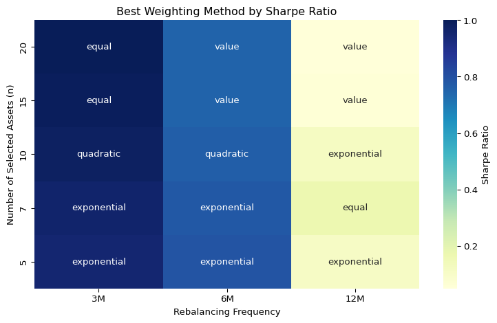

Sharpe Ratio Heatmap (Top-n vs Rebalancing Frequency)

We next examine the impact of rebalancing frequency—specifically, quarterly (3M), semiannual (6M), and annual (12M)—on risk-adjusted performance and underlying portfolio structure. As shown in the heatmap above, quarterly rebalancing tends to produce higher Sharpe ratios across most configurations. However, this benefit comes at the cost of substantially higher turnover. We find that shorter rebalancing intervals better preserve the structural core of TBTF portfolios. Quarterly updates maintain capital concentration and produce stable weight dynamics, while longer horizons may induce drift and dilute structural persistence—especially at larger n.

import seaborn as sns
import matplotlib.pyplot as plt

sns.boxplot(data=turnover_summary_df, x='weighting_method', y='total_turnover', hue='rebalance_freq')
plt.title("Turnover Distribution by Weighting and Frequency")
plt.grid(True)
plt.tight_layout()
plt.show()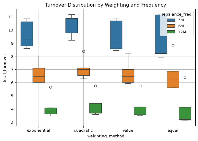

Total Turnover across Parameters

sns.boxplot(
    data=turnover_summary_df,
    x='weighting_method',
    y='total_turnover',
    hue='n'  # Top-n 구성 자산 수
)
plt.title("Turnover Distribution by Weighting and Top-n")
plt.grid(True)
plt.tight_layout()
plt.show()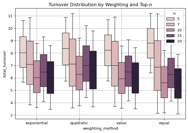

Total Turnover across Parameters

To assess the practical implementability of the TBTF strategy, we examine the total turnover across different weighting schemes and rebalancing frequencies. As illustrated in the boxplot above, turnover levels vary meaningfully by configuration, offering insights into the structural dynamics of each method.

TBTF weighting methods—particularly under less frequent rebalancing (e.g., quarterly or semiannual)—consistently exhibit lower interquartile ranges of turnover, indicating a high degree of structural stability in portfolio composition. In contrast, equal weighting yields the widest dispersion, reflecting more volatile asset entry and reallocation patterns due to its lack of embedded capital sensitivity.

Across all weighting methods, turnover responds strongly to changes in rebalancing frequency. Reducing the frequency from quarterly to semiannual, and from semiannual to annual, results in approximately a twofold decline in average turnover at each step. This regularity highlights a core tradeoff: finer rebalancing intervals enable more timely tracking of short-term shifts but also introduce greater portfolio churn.

A noteworthy exception emerges within the TBTF schemes: quadratic weighting produces higher turnover when moving from semiannual to annual rebalancing—a reversal of the pattern observed in all other methods. This suggests that the quadratic weighting’s greater sensitivity to initial rank–capital structure may amplify reallocations over longer horizons, especially if the top decile membership becomes more volatile at lower rebalancing frequencies.

Taken together, these findings suggest that TBTF-based weighting offers the most stable tradeoff between capital concentration and transaction frictions. In particular, rebalancing at a semiannual or quarterly frequency appears to strike a practical balance, preserving capital lock-in dynamics while keeping turnover at manageable levels.

We further analyze turnover as a function of the number of selected stocks, visualized in the “Turnover Distribution by Weighting and Top-n” plot. Here, TBTF, value-weighted, and equal-weighted portfolios all exhibit their most stable and lowest turnover levels at \(n = 10\) and \(n = 20\). Interestingly, turnover does not decline monotonically as the number of holdings increases. For example, moving from \(n = 10\) to \(n = 15\) slightly increases total turnover before falling again at \(n = 20\). This non-monotonicity suggests that portfolio stability is not simply a function of size, but also of how concentration thresholds interact with the rank dynamics of capital allocation.

# Merge performance & turnover
merged_df = pd.merge(performance_df, turnover_summary_df,
                     on=['n', 'rebalance_freq', 'weighting_method'])

#| fig-cap: "Performance Metric vs. Turnover Tradeoff"
sns.scatterplot(data=merged_df,
                x='total_turnover',
                y='Expected CRRA',
                hue='weighting_method',
                style='rebalance_freq')
plt.title("Performance vs. Turnover Tradeoff")
plt.grid(True)
plt.tight_layout()
plt.show()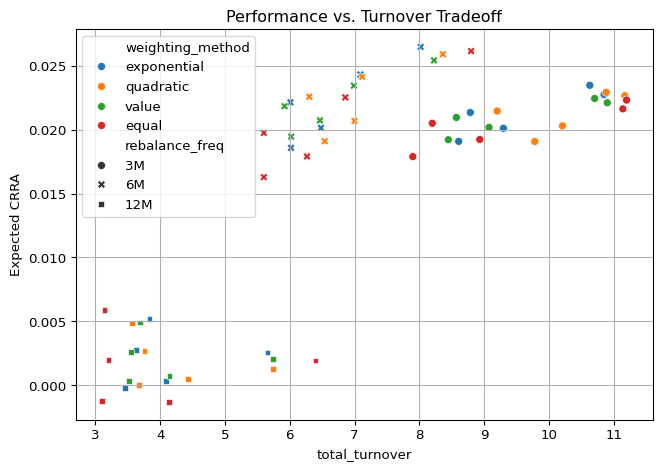

Finally, we visualize the performance-turnover tradeoff, showing how each strategy balances return and implementation frictions:

The figure above visualizes the tradeoff between expected CRRA utility and total turnover across all strategy configurations. Each point represents a unique combination of n, rebalance_freq, and weighting_method.

The resulting plot reveals distinct horizontal clusters by rebalancing frequency, especially under the post-2010 regime. This banding effect is most likely driven by regime-specific shocks—particularly the COVID-19 crash, which had sharply divergent effects depending on the timing of portfolio adjustment.

To further analyze this, we compute the expected CRRA per unit of turnover (i.e., \(\frac{\text{Expected CRRA}}{\text{Total Turnover}}\)) across time subperiods. During non-crisis periods, 6M and 12M configurations yield comparable ratios, with 3M performing slightly lower due to higher turnover. However, during the COVID-19 period, the 6M rebalancing interval dominates, suggesting that it hit a timing sweet spot—being responsive enough to adapt, but not overly reactive like 3M or sluggish like 12M.

These findings underscore the importance of considering macro-structural shocks in assessing turnover efficiency. While quarterly rebalancing ensures persistence and structural alignment, semiannual updates may offer better resilience under nonlinear market stress, at least in crisis regimes.

4 Summary of Robustness

Across a broad set of configurations, the TBTF strategy exhibits strong structural robustness. Its performance remains resilient to changes in portfolio size, weighting method, and rebalancing frequency, indicating that its effectiveness does not hinge on a narrow set of parameter choices.

The consistent superiority of nonlinear weighting schemes—particularly exponential and quadratic—underscores that the TBTF effect stems not merely from large-cap exposure, but from deliberate capital concentration. At the same time, the diminishing performance observed as the number of included assets increases confirms that the strategy draws its strength from a small group of dominant firms at the top of the capital hierarchy.

In implementation terms, both quarterly and semiannual rebalancing strike workable tradeoffs. Quarterly updates better preserve structural lock-in, while semiannual schedules offer greater resilience during regime shocks, such as the COVID-19 episode. Turnover remains moderate in both cases, especially under quadratic weighting, which achieves stability without compromising returns.

Taken together, the evidence suggests that TBTF is neither an artifact of tuning nor a fragile anomaly. Rather, it is a reflection of deeper structural features—platform dominance, passive reinforcement, and institutional persistence—that increasingly govern capital allocation in modern markets.