This section decomposes the structural mechanisms underlying the TBTF strategy across two economic regimes—pre-2010 and post-2010. By comparing these periods, we identify changes in distributional composition, capital concentration, and rank mobility that reflect broader shifts in financial market dynamics following systemic interventions and structural innovation—each of which challenges conventional assumptions in asset pricing and market efficiency.
Code
import numpy as npimport statsmodels.api as smfrom scipy.stats import normfrom sklearn.mixture import GaussianMixtureimport matplotlib.pyplot as pltimport seaborn as sns# CRSP dataframe importimport pandas as pdimport sqlite3con = sqlite3.connect(database="../../tbtf.sqlite")crsp = pd.read_sql_query( sql="SELECT * FROM crsp", con=con, parse_dates={"date"})crsp.head()
permno
date
mktcap
ret
primaryexch
siccd
industry
mktcap_lag
ret_excess
state
state_lag
0
10001
1996-01-31
20.814125
-0.026667
Q
4925
Utilities
21.384375
-0.030967
3
0
1
10001
1996-02-29
21.099250
0.013699
Q
4925
Utilities
20.814125
0.009799
3
3
2
10001
1996-03-31
21.899480
0.036423
Q
4925
Utilities
21.099250
0.032523
3
3
3
10001
1996-04-30
20.348063
-0.070840
Q
4925
Utilities
21.899480
-0.075440
2
3
4
10001
1996-05-31
19.915125
-0.021277
Q
4925
Utilities
20.348063
-0.025477
2
2
1 Mixture Distribution Decomposition
1.1 Core Question:
Is the market portfolio return better explained as a mixture of distinct structural groups, such as top decile vs. the rest, and how have their mixture weights changed across regimes?
1.2 Framework & Method:
We define two return-generating groups:
Group A: Top 10% stocks by market cap (state = 10)
Group B: All other listed stocks (states < 10)
At each month \(t\), compute value-weighted returns:
where \(w_t\) is the capital share of Group A—i.e., the mixture weight.
1.3 Interpretation
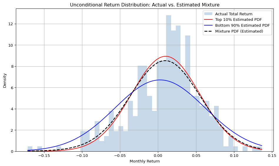
The empirical results from the mixture decomposition provide compelling evidence of a structural shift in how market returns are generated and distributed. Unlike traditional interpretations that focus on regime switching (e.g., bull vs. bear), our analysis reveals a persistent cross-sectional asymmetry—notably between the top decile and the remaining 90% of firms by market capitalization.
Code
# df_miximport numpy as npimport matplotlib.pyplot as plt# 1. Value-Weighted Return 계산 함수 정의def value_weighted_return(df, value_col='mktcap_lag', return_col='ret'): weighted = df[return_col] * df[value_col] total_weight = df[value_col].sum()return weighted.sum() / total_weight if total_weight >0else np.nan# 2. Group별 수익률 계산 및 mixture 분해# 결과 저장용 리스트results = []# 월별 반복for date, group in crsp.groupby('date'): top_group = group[group['state'] ==10] rest_group = group[(group['state'] <10) & (group['state'] >0)]iflen(top_group) ==0orlen(rest_group) ==0:continue# 개별 그룹의 value-weighted return 계산 r_top = value_weighted_return(top_group) r_rest = value_weighted_return(rest_group)# 전체 시장 포트폴리오 value-weighted return 계산 r_total = value_weighted_return(group[group['state'] >0])# mixture weight (자본 비중) w_top = top_group['mktcap_lag'].sum() / group[group['state'] >0]['mktcap_lag'].sum() results.append({'date': date,'r_top': r_top,'r_rest': r_rest,'r_total': r_total,'w_top': w_top,'w_rest': 1- w_top,'r_predicted': w_top * r_top + (1- w_top) * r_rest })df_mix = pd.DataFrame(results).sort_values('date')df_mix.head()
date
r_top
r_rest
r_total
w_top
w_rest
r_predicted
0
1996-01-31
0.034183
-0.003783
0.026941
0.809244
0.190756
0.026941
1
1996-02-29
0.014810
0.027623
0.017185
0.814608
0.185392
0.017185
2
1996-03-31
0.009841
0.017373
0.011246
0.813420
0.186580
0.011246
3
1996-04-30
0.017836
0.056573
0.025221
0.809359
0.190641
0.025221
4
1996-05-31
0.026211
0.034577
0.027858
0.803161
0.196839
0.027858
1.3.1 Capital Lock-In and Mixture Weight Dynamics
Code
# Time-series Capital Weight of Top 10% (State = 10)plt.plot(df_mix['date'], df_mix['w_top'])plt.title('Time-series Capital Weight of Top 10% (State = 10)')plt.xlabel('Date')plt.ylabel('Top 10% Capital Weight')plt.show()
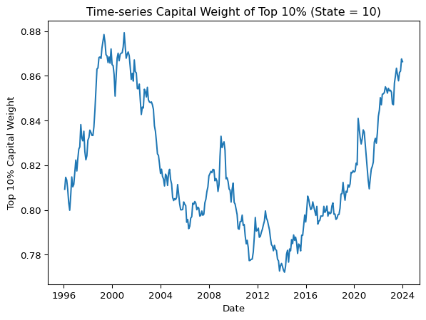
The time-series evolution of \(w_t\)—the value-weighted capital share of the top 10% stocks—offers compelling evidence of persistent and intensifying capital lock-in.
Between 1996 and 2001, \(w_t\) rose rapidly from below 0.75 to a peak of approximately 0.88, reflecting the early stages of mega-cap dominance during the dot-com boom.
After peaking, it declined gradually, reaching just below 0.80 by 2006, indicating a temporary rebalancing of capital across ranks.
From 2006 to 2009, \(w_t\) climbed again, stabilizing around 0.83 during the financial crisis—a period marked by concentrated flight to safety and the early impact of Federal Reserve interventions.
A modest decline occurred post-crisis, with \(w_t\) dipping to around 0.78 in 2011.
Since then, however, the capital share of the top 10% has exhibited near-monotonic increases with remarkably low volatility, except for a brief interruption during the COVID-19 shock in 2020.
By the end of 2023, \(w_t\) had reached levels exceeding 0.85, with persistent upward momentum and minimal fluctuations.
This structural pattern indicates not merely high concentration but capital inertia—a state where capital ceases to reallocate dynamically and instead becomes entrenched within a quasi-permanent elite. Capital flows no longer reflect dynamic responses to fundamentals or risk signals, but instead conform to structural entrenchment supported by indexation, ETF flows, and policy-driven yield compression. Capital lock-in is not only persistent but self-reinforcing, reflecting a transition from competitive allocation to institutionalized dominance.
c.f. Compared to Fama-French’s traditional use of NYSE-only breakpoints, our percentile-based method—spanning NYSE + Nasdaq + AMEX—captures the true cross-sectional concentration of market power, including modern platform firms (e.g., AAPL, MSFT, NVDA) that disproportionately shape returns in the post-crisis era.
1.3.2 Unconditional Return Distributions: Top vs. Rest
Code
# Unconditional Return Distribution: Actual vs. Estimated Mixture# GMM의 간소화 버전" 또는 "semi-parametric mixture modeling# 샘플 수obs =len(df_mix)# 각 그룹의 수익률 평균 및 표준편차r_top_mean = df_mix['r_top'].mean()r_top_std = df_mix['r_top'].std()r_rest_mean = df_mix['r_rest'].mean()r_rest_std = df_mix['r_rest'].std()w_top_mean = df_mix['w_top'].mean()# 실제 및 mixture 수익률r_total = df_mix['r_total']r_predicted = df_mix['r_predicted']# 히스토그램과 PDF x축 범위xmin =min(r_total.min(), r_predicted.min())xmax =max(r_total.max(), r_predicted.max())x = np.linspace(xmin, xmax, 1000)# PDF 계산pdf_top = norm.pdf(x, loc=r_top_mean, scale=r_top_std)pdf_rest = norm.pdf(x, loc=r_rest_mean, scale=r_rest_std)pdf_mix = w_top_mean * pdf_top + (1- w_top_mean) * pdf_rest# Plotplt.figure(figsize=(10, 6))bins = np.linspace(xmin, xmax, 50)# 실제 수익률 히스토그램plt.hist(r_total, bins=bins, alpha=0.3, label='Actual Total Return', color='steelblue', density=True)# 각 컴포넌트 PDFplt.plot(x, pdf_top, linestyle='-', color='red', label='Top 10% Estimated PDF')plt.plot(x, pdf_rest, linestyle='-', color='blue', label='Bottom 90% Estimated PDF')# 혼합 정규 분포 PDFplt.plot(x, pdf_mix, linestyle='--', color='black', linewidth=2, label='Mixture PDF (Estimated)')plt.title("Unconditional Return Distribution: Actual vs. Estimated Mixture")plt.xlabel("Monthly Return")plt.ylabel("Density")plt.legend()plt.grid(True)plt.tight_layout()plt.show()
Code
# Unconditional Return Distribution by Period and Capital Rank Group# 요약 통계 (Pre-2010 vs Post-2010 비교 등)df_mix['period'] = np.where(df_mix['date'] <'2010-01-01', 'Pre-2010', 'Post-2010')# 데이터 재구조화: long formatdf_long = pd.melt( df_mix, id_vars=['date', 'period'], value_vars=['r_top', 'r_rest'], var_name='Group', value_name='Monthly Return')# Group 이름 정리df_long['Group'] = df_long['Group'].replace({'r_top': 'Top 10%','r_rest': 'Bottom 90%'})# Boxplotplt.figure(figsize=(10, 6))sns.boxplot( data=df_long, x='period', y='Monthly Return', hue='Group', palette='Set2')plt.title('Unconditional Return Distribution by Period and Capital Rank Group')plt.axhline(0, color='gray', linestyle='--', linewidth=1)plt.ylabel('Monthly Return')plt.xlabel('Period')plt.legend(title='Group', loc='lower left')plt.tight_layout()plt.show()
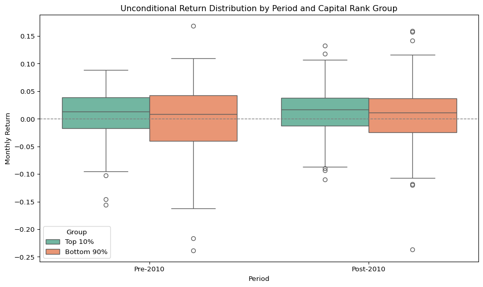
Boxplot visualizations reveal that in the post-2010 regime:
The top decile (r_top) has higher median returns and a narrower interquartile range than the bottom 90% (r_rest).
Outliers on the downside virtually disappear for r_top, while they persist—especially on both tails—for r_rest.
The return distribution of r_top becomes increasingly compact, upward-shifted, and volatility-suppressed, resembling a managed financial product rather than a random equity basket.
These patterns imply that risk-adjusted return asymmetry is not just about mean differences, but about structural volatility suppression and downside risk elimination at the top.
1.3.3 Gaussian Mixture Results: Two-Component Fit
Code
# GMM (k=2) for Top 10% and for Remining 90% import osos.environ['LOKY_MAX_CPU_COUNT'] ='4'# 사용하려는 코어 수를 직접 지정# 각 그룹의 return 시리즈top_returns = df_mix['r_top'].dropna().values.reshape(-1, 1)rest_returns = df_mix['r_rest'].dropna().values.reshape(-1, 1)# GMM 적합 함수def fit_gmm(data, n_components=2): gmm = GaussianMixture(n_components=n_components, random_state=42) gmm.fit(data)return gmmgmm_top = fit_gmm(top_returns, n_components=2)gmm_rest = fit_gmm(rest_returns, n_components=2)def print_gmm_summary(gmm, label):print(f"\nGMM summary for {label}")for i, (w, mu, var) inenumerate(zip(gmm.weights_, gmm.means_, gmm.covariances_)):print(f" Component {i+1}: weight={w:.3f}, mean={mu[0]:.4f}, std={np.sqrt(var[0][0]):.4f}")print_gmm_summary(gmm_top, 'Top 10%')print_gmm_summary(gmm_rest, 'Remaining 90%')
GMM summary for Top 10%
 Component 1: weight=0.290, mean=-0.0307, std=0.0437
 Component 2: weight=0.710, mean=0.0267, std=0.0327

GMM summary for Remaining 90%
 Component 1: weight=0.340, mean=-0.0295, std=0.0750
 Component 2: weight=0.660, mean=0.0193, std=0.0404
The Gaussian Mixture Models (GMMs) estimated separately on r_top and r_rest uncover two key structural regimes:
Both groups exhibit bimodal structure, with one cluster capturing low-mean, high-volatility returns, and the other positive-mean, low-volatility returns.
However, for the top decile, the low-return regime has a lower weight and tighter variance, suggesting that even when shocks occur, they are attenuated within this elite group.
In contrast, the bottom 90% remains exposed to broader volatility regimes, maintaining a larger spread of possible outcomes.
1.3.4 Testing Internal Heterogeneity in Top Decile
Code
# k Selection by AIC vs. BICX = df_mix['r_top'].dropna().values.reshape(-1, 1)aic_scores = []bic_scores = []ks =range(1, 21)for k in ks: gmm = GaussianMixture(n_components=k, random_state=42) gmm.fit(X) aic_scores.append(gmm.aic(X)) bic_scores.append(gmm.bic(X))# Plot AIC vs BIC to visualize optimal kplt.plot(ks, aic_scores, label='AIC')plt.plot(ks, bic_scores, label='BIC')plt.xlabel('Number of Components (k)')plt.ylabel('Information Criterion')plt.legend()plt.title('Model Selection: AIC vs BIC')plt.grid(True)plt.show()
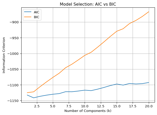
To test whether the top decile itself contains further latent substructures, we estimate GMMs with increasing number of components (\(k = 1, 2, ..., 20\)). The result is striking:
Both AIC and BIC increase monotonically in \(k\), indicating that no additional latent components significantly improve model fit.
The most parsimonious and interpretable solution is obtained at \(k = 2\) or even \(k = 1\), reinforcing the view that a single dominant structural cluster governs return generation at the top.
This suggests that return asymmetry may not stem from overlapping regimes or transitory factors, but rather from the structural dominance of a statistically persistent subgroup of mega-cap firms.
1.4 Summary Interpretation
Together, these results imply that:
The top-decile portfolio behaves like a capital sink—absorbing flows while insulating itself from market volatility.
Market return is no longer the outcome of dispersed competition, but rather converges to a structurally locked elite, supported by policy, passive flows, and indexation mechanics.
This undermines the classical view of a dynamic, risk-compensated market and instead points toward structural rent extraction by the few.
2 Capital Share Convexity: Quadratic Regression Evolution
2.1 Core Question:
Has capital become more concentrated in the top-ranked firms over time?
where \(\text{Rank}_i\) is percentile-based with state 1 = bottom 10%, …, state 10 = top 10%.
The convexity of capital distribution is captured by \(\gamma_t\):
\(\gamma_t > 0\) implies increasing convexity, or accelerated capital share at the top.
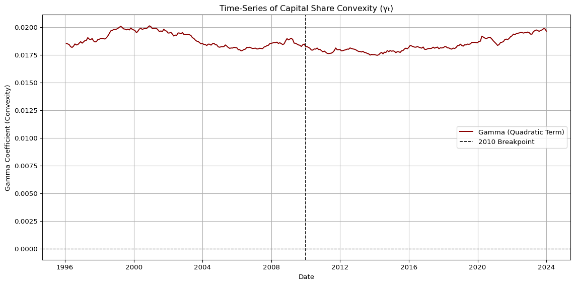
Time-series \(\{\gamma_t\}\) is visualized to show evolution of capital inequality.
2.3 Interpretation
Code
# Time-Series of Capital Share Convexity# 1. 각 날짜별로 state별 mktcap 합산 → CapShare_i 생성def compute_capshare(df): df = df.copy() cap_by_state = df.groupby('state')['mktcap'].sum() total_cap = cap_by_state.sum() df['cap_share'] = df['state'].map(cap_by_state / total_cap)return df# 2. cross-sectional regression에서 사용될 state별 요약 데이터 생성def compute_quadratic_coefficients(df): results = []for date, group in df.groupby('date'):# 유효한 state만 사용 (state 0은 제외) group = group[group['state'] >0].copy() cap_by_state = group.groupby('state')['mktcap'].sum() total_cap = cap_by_state.sum() capshare = cap_by_state / total_cap# x = state (1~10), y = capshare x = capshare.index.values y = capshare.values X = np.column_stack([x, x**2]) X = sm.add_constant(X) model = sm.OLS(y, X).fit() results.append({'date': date,'alpha': model.params[0],'beta': model.params[1],'gamma': model.params[2],'r_squared': model.rsquared })return pd.DataFrame(results)def plot_gamma_time_series(gamma_df): plt.figure(figsize=(12, 6)) plt.plot(gamma_df['date'], gamma_df['gamma'], label='Gamma (Quadratic Term)', color='darkred')# 기준선들 plt.axhline(0, color='gray', linestyle='--', linewidth=1) plt.axvline(pd.to_datetime("2010-01-01"), color='black', linestyle='--', linewidth=1.2, label='2010 Breakpoint') plt.title('Time-Series of Capital Share Convexity (γₜ)') plt.xlabel('Date') plt.ylabel('Gamma Coefficient (Convexity)') plt.legend() plt.grid(True) plt.tight_layout() plt.show()crsp_filtered = crsp[crsp['state'] >0].copy()gamma_df = compute_quadratic_coefficients(crsp_filtered)plot_gamma_time_series(gamma_df)
The time-series of the capital share convexity coefficient, \(\gamma_t\), estimated via cross-sectional quadratic regressions, reveals a striking and persistent structure.
Code
gamma_df.drop('date', axis=1).describe()
alpha
beta
gamma
r_squared
count
336.000000
336.000000
336.000000
336.000000
mean
0.234058
-0.154610
0.018605
0.669198
std
0.010872
0.006820
0.000692
0.015498
min
0.215743
-0.169420
0.017445
0.635521
25%
0.225711
-0.160178
0.018074
0.656935
50%
0.231705
-0.152995
0.018444
0.672377
75%
0.242551
-0.149454
0.019180
0.681382
max
0.257679
-0.143156
0.020107
0.695882
Across the full sample period (1996–2023), \(\gamma_t\) remains consistently positive and tightly bounded, with:
A mean value of approximately 0.0186,
A narrow interquartile range: [0.0181, 0.0192],
A low standard deviation of 0.0007, and
R-squared values averaging 0.67, indicating robust fit quality across time.
This remarkable temporal consistency suggests that the top ranks in the market-cap distribution have maintained a structurally convex advantage—absorbing disproportionately higher capital relative to their rank in nearly every month over the past three decades.
A closer examination shows that:
Prior to 2010, there was mild downward drift in \(\gamma_t\), consistent with episodic rebalancing and potential capital redistribution (e.g., during the post-dotcom or pre-GFC phase).
However, post-2010, \(\gamma_t\) exhibits a slight but stable upward trend, indicating reinforced convexity—a steeper capital concentration curve among the top-ranked firms.
This empirical curvature echoes the shape of a discrete Lorenz curve, where \(\gamma_t\) can be interpreted as a “capital inequality curvature index”. In this framework, increases in \(\gamma_t\) correspond to a more extreme dominance of top ranks, consistent with both the capital lock-in and transition persistence mechanisms documented elsewhere in this study.
Importantly, the tight dispersion and monotonic stabilization of \(\gamma_t\) provide indirect but compelling support for the out-of-sample consistency of capital-weight-based strategies. The fact that the quadratic relationship between rank and capshare is not only convex but also time-invariant implies that a convex weighting scheme calibrated in-sample may remain optimal (or near-optimal) out-of-sample.
This further reinforces the central hypothesis of the TBTF framework: top capital positions are not merely episodic outcomes but persistent structural anchors in modern financial markets.
3 Persistence and Lock-In Dynamics
좋습니다. 아래는 4_4_structure.qmd의 “Persistence and Lock-In Dynamics” 섹션 중, Markov transition matrix 추정 방식을 실제 구현된 10×10 matrix 기반으로 수정 및 보완한 내용입니다. 핵심은 다음 두 가지입니다:
원래 open system에서 state = 0(탈락 또는 미관측 상태)을 포함한 11×11 matrix는 완전히 닫힌 체계(closed system)가 아님
본 분석은 실용적 접근으로 state = 1–10 범위에만 집중한 pseudo-closed system으로 제한하고, 이에 따른 해석상의 제약은 추후 확장 연구로 남긴다는 코멘트를 명시
4 Persistence and Lock-In Dynamics
4.1 Core Question:
Is capital mobility declining, with firms increasingly locked in to top positions?
4.2 Framework & Method
States are defined as decile ranks of market capitalization:
State 10: Top 10% (≥ 90th percentile)
States 6–9: Upper middle 40% (50–90 percentile)
States 1–5: Bottom 50%
State 0: Delisted or unranked (excluded from main estimation)
Using CRSP panel data, we construct an empirical first-order Markov transition matrix:
The original system includes state 0, representing delisting or unranked stocks.
However, to focus on the relative dynamics of ranked firms and avoid structural imbalance caused by market entry/exit, we restrict the analysis to states 1–10, forming a pseudo-closed system.
This restriction implicitly conditions on survival and omits net capital flow into or out of the system.
A more comprehensive treatment including open-system dynamics (e.g., absorbing states, boundary flows) is deferred to future work.
We estimate:
The 10×10 transition matrix \(P_{ij}\) among ranked states only.
Diagonal elements (\(P_{ii}\)): Represent state persistence or retention probability.
Off-diagonal elements: Capture mobility dynamics, including upward or downward shifts.
The stationary distribution\(\pi\) is computed via eigen decomposition:
\[
\pi' P = \pi', \quad \sum_i \pi_i = 1
\]
All transition counts are computed from actual firm-level changes in decile state based on monthly data, pre-processed to include both listing and delisting effects via augmented panel construction (crsp_trunc).
4.3 Interpretation
Code
import sysimport os# 현재 경로 기준으로 상위 디렉토리로 경로 추가sys.path.append(os.path.abspath('../..'))import tbtf_dataff3 = tbtf_data.load_ff3_factors(start_date=crsp['date'].min(), end_date=crsp['date'].max())crsp_trunc = tbtf_data.crsp_truncation(crsp,ff3)# crsp_full = tbtf_data.crsp_lifecycle(crsp_trunc)
Code
# ================================================# transition_matrix : pd.DataFrame (10x10)# stationary_series : pd.Series (length 10)# ================================================# old-living만 선택 (full lifecycle이 없거나 right-truncated)#crsp_valid = crsp_full[crsp_full['lifetype'] == 'old-living'].copy()#print("The number of stocks from state 0 to any states:", (crsp_trunc['state_lag'] == 0).sum())#print("The number of stocks from any states to state 0:", (crsp_trunc['state'] == 0).sum())#print("The number of Total In-flow stocks during the sample period:", (crsp_trunc['state_lag'] == 0).sum()-(crsp_trunc['state'] == 0).sum())# Transition matrix 계산 시점에서 filtering# 조건: state_lag ∈ [1, 10] AND state ∈ [1, 10]crsp_valid = crsp_trunc.query("state > 0 and state_lag > 0").copy()# Compute empirical transition counts# (state_lag → state) pair frequency tabletransition_counts = ( crsp_valid .groupby(['state_lag', 'state']) .size() .unstack(fill_value=0) .sort_index() .reindex(columns=range(1, 11), fill_value=0) # Ensure all states 0 to 10 are present)# Convert counts to row-wise probabilities# Each row represents conditional distribution: P(next state | current state)transition_matrix = transition_counts.div(transition_counts.sum(axis=1), axis=0)# Compute stationary distribution (long-run equilibrium distribution over states)# Method: Use eigen-decomposition of the transpose of the transition matrixeigvals, eigvecs = np.linalg.eig(transition_matrix.T.values)stationary = np.real(eigvecs[:, np.isclose(eigvals, 1)])# Normalize to sum to 1stationary = stationary[:, 0]stationary_dist = stationary / stationary.sum()# Format for outputtransition_matrix.index.name ='From State'transition_matrix.columns.name ='To State'stationary_series = pd.Series(stationary_dist, index=transition_matrix.columns, name='Stationary Dist.')# Markov Transition Matrix Heatmap (States 0–10)import seaborn as snsplt.figure(figsize=(10, 8))sns.heatmap( transition_matrix, annot=True, fmt=".3f", cmap="YlGnBu", linewidths=0.5, cbar_kws={'label': 'Transition Probability'}, xticklabels=[f"To {i}"for i in transition_matrix.columns], yticklabels=[f"From {i}"for i in transition_matrix.index])plt.title("Markov Transition Matrix Heatmap (States 0–10)")plt.xlabel("Next Period State")plt.ylabel("Current Period State")plt.tight_layout()plt.show()
Code
# Long-Run Stationary Distribution by State (Excl. Exit)# Step 4: Compute stationary distribution# Method: Use eigen decomposition for the transpose of the transition matrixeigvals, eigvecs = np.linalg.eig(transition_matrix.T.values)stationary = np.real(eigvecs[:, np.isclose(eigvals, 1)])stationary = stationary[:, 0]stationary_dist = stationary / stationary.sum()# Prepare final transition matrix and stationary distributiontransition_matrix.index.name ='From State'transition_matrix.columns.name ='To State'stationary_series = pd.Series(stationary_dist, index=transition_matrix.columns, name="Stationary Dist.")# State 1부터 10까지의 stationary probabilitystationary_series_nonzero = stationary_series.iloc[:]# Plotplt.figure(figsize=(8, 5))sns.barplot( x=stationary_series_nonzero.index.astype(str), y=stationary_series_nonzero.values, color='steelblue', edgecolor='black')# Annotate each bar with its valuefor i, val inenumerate(stationary_series_nonzero.values): plt.text(i, val +0.001, f"{val:.3f}", ha='center', va='bottom', fontsize=10)# Plot labels and formattingplt.title("Long-Run Stationary Distribution by State (Excl. Exit)", fontsize=14)plt.xlabel("State (Market Cap Rank)", fontsize=12)plt.ylabel("Stationary Probability", fontsize=12)plt.xticks(rotation=0)plt.ylim(0, stationary_series_nonzero.max() +0.01)plt.tight_layout()plt.show()
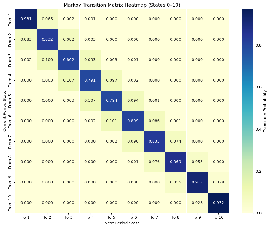
The estimated Markov transition matrix and stationary distribution, constructed using only ranked states (States 1–10), reveal a structurally persistent yet more symmetric capital mobility structure than previously observed in open-system models that included State 0. By excluding delisted or unranked firms, this framework focuses on rank-to-rank transitions within the surviving universe of firms and captures a distinct form of intra-market hierarchy.
High Persistence at the Extremes
The system continues to exhibit strong persistence at both ends of the distribution. In particular, the top decile (State 10) shows a self-transition probability of 0.972, implying an expected duration of over 36 months. This persistence confirms that once firms enter the top decile, they tend to remain there, reinforcing the notion that the highest tier functions as a quasi-absorbing state.
Similarly, the bottom decile (State 1) displays a self-transition probability of 0.931, also associated with prolonged durations. This bilateral persistence at the extremes suggests a structural form of capital stratification, where firms, once classified into the highest or lowest decile, tend to stay put. These two tails behave like boundary layers of the rank system, characterized by entrenchment rather than fluid mobility.
Mobility in the Middle
In contrast, the middle states—especially States 4 and 5—display the lowest persistence, each with a diagonal transition probability near 0.79. These intermediate ranks represent the most unstable region of the system, acting as a transitory buffer between the stable top and bottom groups. Firms in these states face greater uncertainty and classification volatility, neither entrenched like the top-tier incumbents nor consistently relegated like small-cap firms.
This suggests that mid-cap firms are most exposed to competitive reshuffling. Their trajectories remain open-ended, with material probabilities of upward or downward movement depending on performance shocks or relative repricing, but with limited protection from persistent identity.
Absence of Exit/Entry Mechanisms
In this formulation, the Markov chain excludes transitions into or out of State 0. As such, delisting and new entries are not explicitly modeled. This simplification defines a pseudo-closed system designed to examine intra-system mobility rather than open-market turnover. The exclusion of exit risk makes the estimated transition probabilities purely conditional on being within the ranked universe, ideal for studying relative capital stickiness but less suited for estimating attrition or survivorship.
This design choice removes the asymmetry introduced by non-reversible states such as delisting or IPO-based entry, which would otherwise distort the symmetry of the estimated chain. While this comes at the cost of completeness, it offers clarity in isolating the structural dynamics of persistence, volatility, and mobility within the active market.
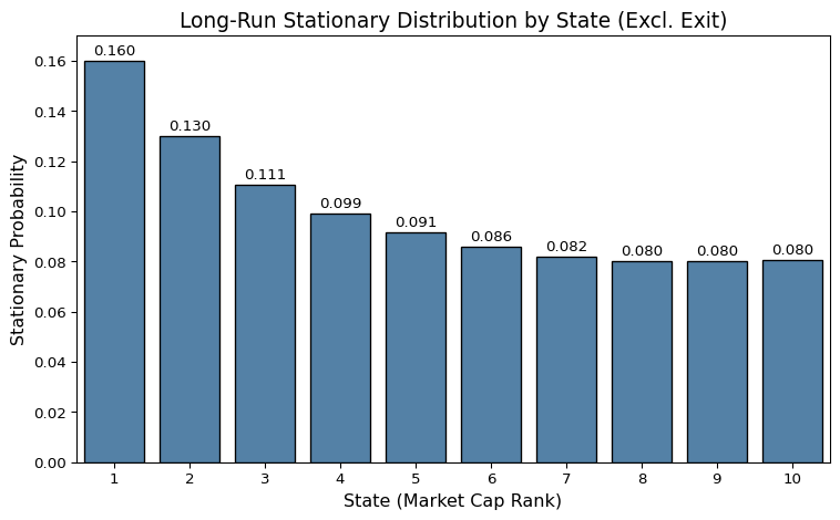
The estimated stationary distribution across ranked states displays a gradual but consistent decline from lower to higher ranks. State 1 exhibits the highest long-run probability, at approximately 16 percent, while State 10 stabilizes at around 8 percent. This pattern suggests that lower-ranked firms are more prevalent in the long run, at least in terms of count, even though they may not dominate capital or influence.
Two forces likely drive this skew: first, a disproportionately high entry frequency into the lower deciles, often from new listings or small restructurings; and second, a limited degree of upward mobility from these initial positions. The bottom deciles, while not formally absorbing, act as a sticky floor—consistently replenished by inflows yet rarely exited by transitions to higher states.
The implication is that mobility across ranks is asymmetric even within the active market. Structural regeneration happens predominantly at the bottom, while upward reallocation remains limited. This reinforces the interpretation of the capital market not as a fluid mobility engine, but as a system with hierarchical layers, each marked by different persistence dynamics and long-run outcomes.
5 Summary Table
Structural Channel
Mechanism
Interpretation
Mixture
Return as weighted sum of 2 subgroups
Top decile increasingly drives aggregate performance
Convexity
Capital share as function of rank
Lorenz-type concentration intensifies over time
Transition
Markov dynamics of rank-state mobility
Top and Exit states are quasi-absorbing, path-dependent
Top-decile persistence reveals a form of quasi-absorption, where firms not only rise to the top but stay there disproportionately longer — effectively becoming “Too Big to Exit.”
Middle-rank volatility suggests structural fragility, with firms unable to stabilize or ascend — reflecting a “Fragile Middle” that lacks lasting competitive foothold.
Lower-rank saturation reflects systemic bottlenecks, where inflows into low deciles are not matched by upward mobility — indicating a “sticky floor” rather than an active ladder.
The long-run distribution reinforces this structure: capital is not symmetrically mobile, but increasingly trapped in persistent states. This challenges foundational assumptions in representative-agent models, suggesting instead that capital flows in financial markets obey a hierarchical and inertial logic, not a fluid or ergodic one.