Code
import numpy as np
import pandas as pd
import sqlite3
con = sqlite3.connect(database="../../tbtf.sqlite")

crsp = pd.read_sql_query(
  sql="SELECT * FROM crsp",
  con=con,
  parse_dates={"date"}
)Traditional asset pricing frameworks rest on no-arbitrage principles and risk-return tradeoffs, assuming that all assets exist to offer compensation for exposure to priced risks. Under such models, individual asset returns are interpreted as linear functions of sensitivities to systematic risk factors.
In contrast, the TBTF (Too Big To Fail) strategy is motivated by a fundamentally different view of financial markets under late-stage capitalism. We argue that the secondary stock market reflects persistent dominance by a small subset of firms whose market power is self-reinforcing. These firms attract new capital not due to risk-efficiency, but due to narrative-driven legitimacy and path-dependent concentration of initial endowment.
This motivates a strategy grounded not in diversification or risk exposure, but in capital persistence, market lock-in, and capital hierarchy.
The TBTF strategy is constructed under When-What–How framework:
Our strategy operates on the full set of U.S. listed common stocks traded on NYSE, NASDAQ, and AMEX. Stocks with non-positive market capitalization are excluded to avoid bankrupt or illiquid firms.
import numpy as np
import pandas as pd
import sqlite3
con = sqlite3.connect(database="../../tbtf.sqlite")
crsp = pd.read_sql_query(
sql="SELECT * FROM crsp",
con=con,
parse_dates={"date"}
)Each month, firms are ranked by market capitalization. These rankings define discrete capital states (percentile bins). We focus on the top-decile (state = 10), selecting the top-\(n\) firms at time \(t\) based on market-cap rank. The baseline is \(n=10\), with robustness checks for \(n \in \{5, 7, 10, 15, 20\}\).
A Markovian state transition framework is imposed to capture the temporal dynamics of capital flow between ranked states. The top state exhibits persistent and asymmetric capital retention, supporting the capital lock-in hypothesis.
We evaluate several portfolio weighting methods:
TBTF (Convex Structural Weighting):
Capital weights are determined by in-sample estimates of the convex relationship between market-cap rank and capital share. For example, specifications can be :
Note that the exponential form ensures structural monotonicity.
Value-Weighted (VW):
Proportional to each firm’s market capitalization.
Equal-Weighted (EQ):
Uniform allocation across all selected assets.
import matplotlib.pyplot as plt
import seaborn as sns

# 현재 경로 기준으로 상위 디렉토리로 경로 추가
import sys, os
sys.path.append(os.path.abspath('../..'))

import tbtf
To empirically validate the structural weighting functions, we fit several models to the in-sample relationship between rank and capital share. The following plots show the cross-sectional fitting results based on a representative rebalance date.
in_end = '2009-12-31'
in_sample_months = 48

print('Snapshot at:', in_end)
print('Look-back period:', in_sample_months, 'months')

df_in_sample, _ = tbtf.split_in_out_sample(crsp, in_end, in_sample_months)
Snapshot at: 2009-12-31
Look-back period: 48 monthsfig, axes = plt.subplots(3, 2, figsize=(14, 15))
tbtf.plot_quadratic_fit(df_in_sample, n=10, state=10, ax=axes[0, 0])
tbtf.plot_exponential_fit(df_in_sample, n=10, state=10, ax=axes[0, 1])
tbtf.plot_mean_fit(df_in_sample, n=10, state=10, ax=axes[1, 0])
tbtf.plot_loess_fit(df_in_sample, n=10, state=10, ax=axes[1, 1])
tbtf.plot_bayes_fit(df_in_sample, n=10, state=10, ax=axes[2, 0])
tbtf.plot_spline_fit(df_in_sample, n=10, state=10, ax=axes[2, 1])
fig.suptitle(f"Fitted Capital Share Functions at {in_end}", fontsize=16)
plt.tight_layout()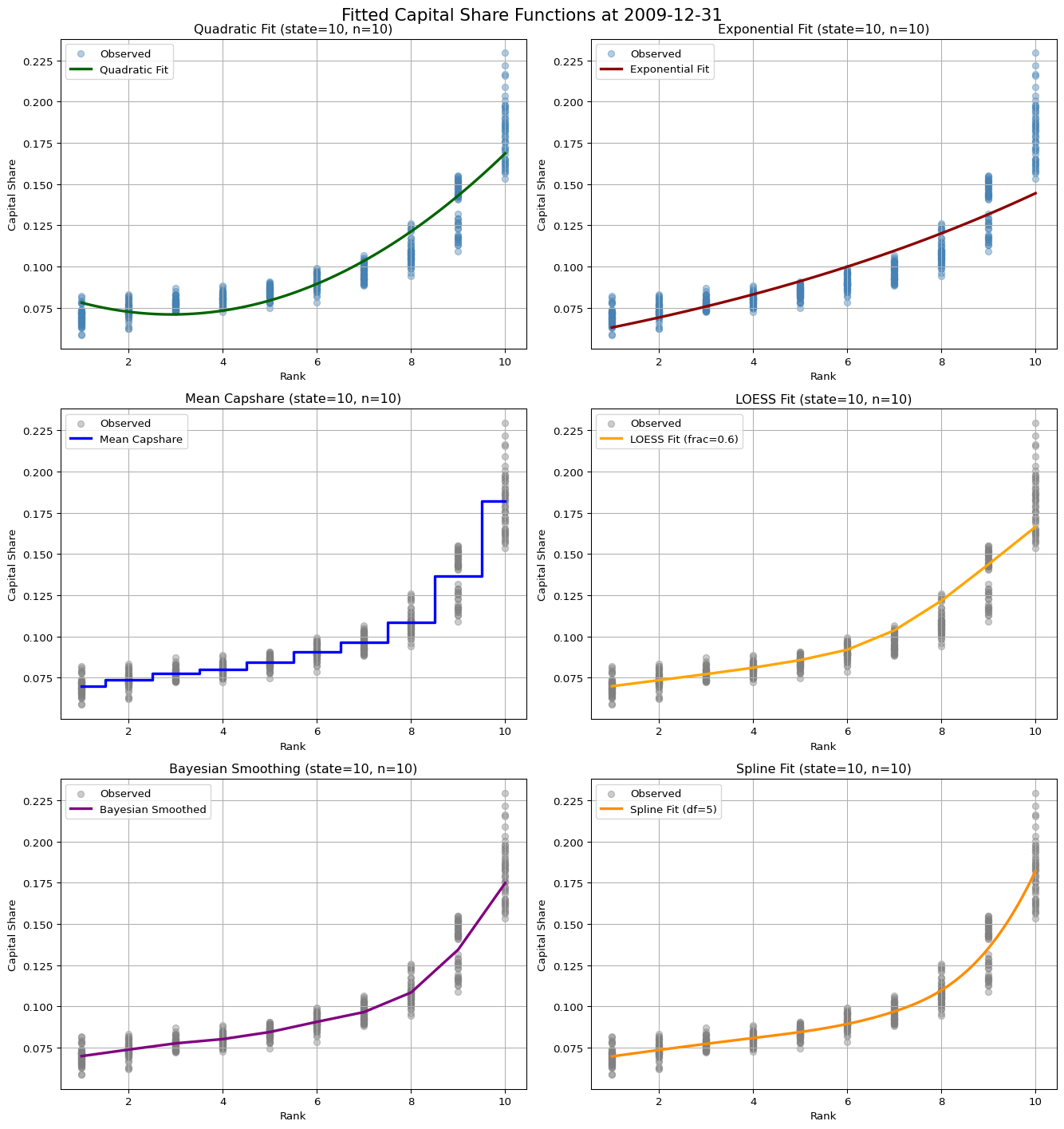
in_end = '2023-12-31'
in_sample_months = 48

print('Snapshot at:', in_end)
print('Look-back period:', in_sample_months, 'months')

df_in_sample, _ = tbtf.split_in_out_sample(crsp, in_end, in_sample_months)
Snapshot at: 2023-12-31
Look-back period: 48 monthsfig, axes = plt.subplots(3, 2, figsize=(14, 15))
tbtf.plot_quadratic_fit(df_in_sample, n=10, state=10, ax=axes[0, 0])
tbtf.plot_exponential_fit(df_in_sample, n=10, state=10, ax=axes[0, 1])
tbtf.plot_mean_fit(df_in_sample, n=10, state=10, ax=axes[1, 0])
tbtf.plot_loess_fit(df_in_sample, n=10, state=10, ax=axes[1, 1])
tbtf.plot_bayes_fit(df_in_sample, n=10, state=10, ax=axes[2, 0])
tbtf.plot_spline_fit(df_in_sample, n=10, state=10, ax=axes[2, 1])
fig.suptitle(f"Fitted Capital Share Functions at {in_end}", fontsize=16)
plt.tight_layout()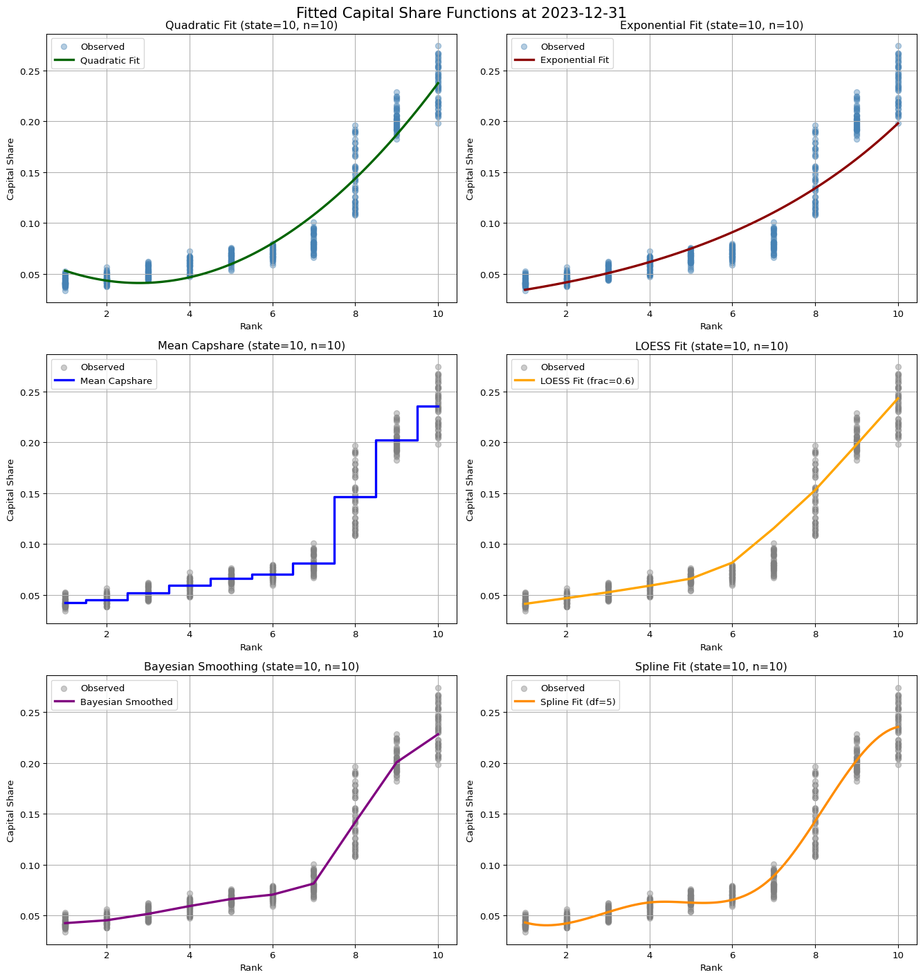
We test fixed-interval rebalancing schemes:
Rebalancing frequency directly affects turnover and transaction cost implications. Monthly rebalancing is selected as the baseline to balance responsiveness with frictions.
For external comparison, we use:
The TBTF strategy is not merely a rule-based selection method. It reflects a structural argument that allocative efficiency in modern markets is compromised by persistent capital concentration. Instead of diversifying away idiosyncratic risk, markets are increasingly dominated by capital lock-in, hierarchy reinforcement, and narrative legitimacy.
This framework reconceptualizes the role of financial assets from carriers of risk to vehicles of structural dominance, and evaluates portfolio construction in light of this altered paradigm.
This appendix section outlines the modular structure of the TBTF portfolio strategy, from input specification to out-of-sample return generation and performance evaluation. The pipeline is designed to be flexible across different weighting schemes, rebalance frequencies, and strategy parameters.
| Argument | Description |
|---|---|
df |
Main input DataFrame (crsp) including fields such as date, permno, mktcap, ret, state, mktcap_lag, etc. |
state_level |
Target capital state to define the asset universe, typically the top decile (e.g., 10). |
top_n |
Number of assets to be selected at each rebalance point (e.g., n ∈ {5, 10, 20, 30, 50}). |
rebalance_freq |
Rebalancing interval (e.g., '1M', '3M', '6M', '12M'). |
weighting_method |
One of 'equal', 'value', 'quadratic', or 'exponential'. |
in_sample_period |
Estimation window for in-sample weight calibration (e.g., '2010-01-01' to '2013-12-31'). |
out_sample_period |
Evaluation window for out-of-sample backtesting (e.g., '2014-01-01' to '2023-12-31'). |
eta, p |
Parameters for CRRA utility (eta) and Omega ratio threshold (p). |
in_sample = df[(df['date'] >= in_sample_start) & (df['date'] <= in_sample_end)]
out_sample = df[(df['date'] > in_sample_end) & (df['date'] <= out_sample_end)]
universe = df[df['state'] == state_level]If weighting_method is 'quadratic' or 'exponential':
Estimate the relationship between within-state rank and capital share using in-sample data:
Save estimated coefficients:
coefficients = {'alpha': ..., 'beta': ..., 'gamma': ...}For each rebalance date in the out-sample period:
state == state_level)n[date, permno, weight] for forward return applicationAt each evaluation date after rebalance:
For each rebalance window:
Using out-of-sample return series, compute:
Risk-Adjusted Metrics:
p)etaReturn summary as dictionary:
metrics_dict = {
    'Sharpe': ...,
    'Sortino': ...,
    'Omega': ...,
    'CRRA': ...,
    'CAGR': ...,
    'MDD': ...
}| Output | Description |
|---|---|
returns_df |
Time series of out-of-sample portfolio returns |
weights_df |
Portfolio composition (weights per date and permno) |
turnover_df |
Time series of turnover at each rebalance point |
metrics_dict |
Dictionary of strategy performance metrics |
#| label: TBTF Strategy Full Module
#| warning: false
#| message: false

import pandas as pd
import numpy as np
import statsmodels.api as sm

# ----------------------------
# 1. Data Partitioning
# ----------------------------
def split_in_out_sample(df, in_end, in_sample_months=36, out_end=None):
    in_sample = df[(df['date'] <= in_end)].copy()
    if out_end:
        out_sample = df[(df['date'] > in_end) & (df['date'] <= out_end)].copy()
    else:
        out_sample = df[(df['date'] > in_end)].copy()
    return in_sample, out_sample

# ----------------------------
# 2. Weight Estimation
# ----------------------------
def estimate_exponential_weights(df_in_sample, n=10, state=10):
    # Placeholder for full implementation
    pass

def estimate_quadratic_weights(df_in_sample, n=10, state=10):
    # Placeholder for full implementation
    pass
# ----------------------------
# 3. Portfolio Construction
# ----------------------------
def construct_tbtf_exponential(crsp_df, target_state, top_n, params):
    # Placeholder for full implementation
    pass

def construct_tbtf_quadratic(crsp_df, target_state, top_n, params):
    # Placeholder for full implementation
    pass

# ----------------------------
# 4. Return and Turnover Calculation
# ----------------------------
def compute_return_tbtf(crsp, rebalance_dates, weighting_method='exponential', top_n=10, state=10, in_sample_months=36):
    # Placeholder for full implementation
    pass

def compute_return_pfo(crsp, rebalance_dates, weighting_method='vw', top_n=10):
    # Placeholder for traditional VW or EW method
    pass

def compute_turnover(weights_df, rebalance_dates):
    # Placeholder for full implementation
    pass

# ----------------------------
# 5. Performance Evaluation
# ----------------------------
def evaluate_performance(returns, eta=3, p=0.01, periods_per_year=12):
    # Placeholder for full implementation
    pass

# ----------------------------
# 6. Rebalance Date Utility
# ----------------------------
def get_rebalance_offset(rebalance_freq):
    # Placeholder for full implementation
    pass

# ----------------------------
# 7. Backtest Pipeline
# ----------------------------
def backtest_pipeline(crsp, in_end, out_end, in_sample_months, rebalance_freq, weighting_method, top_n, state, eta, p):
    # Placeholder for full backtest execution logic
    pass

# ----------------------------
# 8. Visualization (optional)
# ----------------------------
def plot_quadratic_fit(df_in_sample, n=10, state=10):
    # Placeholder for plot generation
    pass

def plot_exponential_fit(df_in_sample, n=10, state=10):
    # Placeholder for plot generation
pass| Method | Functional Form | Statistical Interpretation | Flexibility | Stability | Interpretability | Complexity |
|---|---|---|---|---|---|---|
| Mean-Based | Stepwise function | Group-wise Sample Mean | Low | Low | High | Very Low |
| LOESS | Local smoothing | Nonparametric Local Regression | Very High | Medium | Medium | Moderate |
| Bayesian | Global shrinkage estimator | Hierarchical Bayesian Model | Medium | High | Medium | Moderate–High |
| Spline | Smooth piecewise polynomial | Semi-parametric Regression | High | Medium | Medium | Moderate |
Definition
For each rank \(r \in \{1,\dots,10\}\), we estimate the average capital share over the in-sample period: \[
\hat{w}_r = \frac{1}{T} \sum_{t=1}^{T} w_{r,t}
\]
Statistical Structure
Theoretical Interpretation
Advantages
Limitations
Definition
Capital share is estimated via local regression, using a kernel-weighted average of nearby observations: \[
\hat{w}_r = \sum_{j} K\left(\frac{r - j}{h}\right) w_j
\] - \(K(\cdot)\) is a kernel function (e.g., tricube); \(h\) controls the bandwidth and smoothness.
Statistical Structure
Theoretical Interpretation
Advantages
Limitations
Definition
Each rank-specific capital share \(w_r\) is modeled as a noisy observation from a latent distribution: \[
w_r \sim \mathcal{N}(\theta_r, \sigma_r^2), \quad \theta_r \sim \mathcal{N}(\mu, \tau^2)
\]
Statistical Structure
Theoretical Interpretation
Advantages
Limitations
Definition
The rank–capshare function is approximated as a linear combination of spline basis functions: \[
\hat{w}_r = \sum_{k} \beta_k B_k(r)
\] - \(B_k(r)\) are spline basis functions (e.g., B-splines or natural splines).
Statistical Structure
Theoretical Interpretation
Advantages
Limitations